What Is Power?

Angela L.E. Walmsley and Michael C. Brown, Concordia University Wisconsin

For many teachers of introductory statistics, power is a concept that is often not used. In many cases, it’s avoided altogether. In fact, many Advanced Placement (AP) teachers stay away from the topic when they teach tests of significance, according to Floyd Bullard in “Power in Tests of Significance.” However, power is an important concept to understand as a consumer of research, no matter what field or profession a student may enter as an adult. Hence, discussion of power should be included in an introductory course.

To discuss and understand power, one must be clear on the concepts of Type I and Type II errors. Doug Rush provides a refresher on Type I and Type II errors (including power and effect size) in the Spring 2015 issue of the Statistics Teacher Network, but, briefly, a Type I Error is rejecting the null hypothesis in favor of a false alternative hypothesis, and a Type II Error is failing to reject a false null hypothesis in favor of a true alternative hypothesis. The probability of a Type I error is typically known as Alpha, while the probability of a Type II error is typically known as Beta.

Now on to power. Many learners need to be exposed to a variety of perspectives on the definition of power. Bullard describes multiple ways to interpret power correctly:

• Power is the probability of rejecting the null hypothesis when, in fact, it is false.
• Power is the probability of making a correct decision (to reject the null hypothesis) when the null hypothesis is false.
• Power is the probability that a test of significance will pick up on an effect that is present.
• Power is the probability that a test of significance will detect a deviation from the null hypothesis, should such a deviation exist.
• Power is the probability of avoiding a Type II error.

Simply put, power is the probability of not making a Type II error, according to Neil Weiss in Introductory Statistics.

Mathematically, power is 1 – beta. The power of a hypothesis test is between 0 and 1; if the power is close to 1, the hypothesis test is very good at detecting a false null hypothesis. Beta is commonly set at 0.2, but may be set by the researchers to be smaller.

Consequently, power may be as low as 0.8, but may be higher. Powers lower than 0.8, while not impossible, would typically be considered too low for most areas of research.

Bullard also states there are the following four primary factors affecting power:

1. Significance level (or alpha)
2. Sample size
3. Variability, or variance, in the measured response variable
4. Magnitude of the effect of the variable

Power is increased when a researcher increases sample size, as well as when a researcher increases effect sizes and significance levels. There are other variables that also influence power, including variance (σ2), but we’ll limit our conversation to the relationships among power, sample size, effect size, and alpha for this discussion.

In reality, a researcher wants both Type I and Type II errors to be small. In terms of significance level and power, Weiss says this means we want a small significance level (close to 0) and a large power (close to 1).

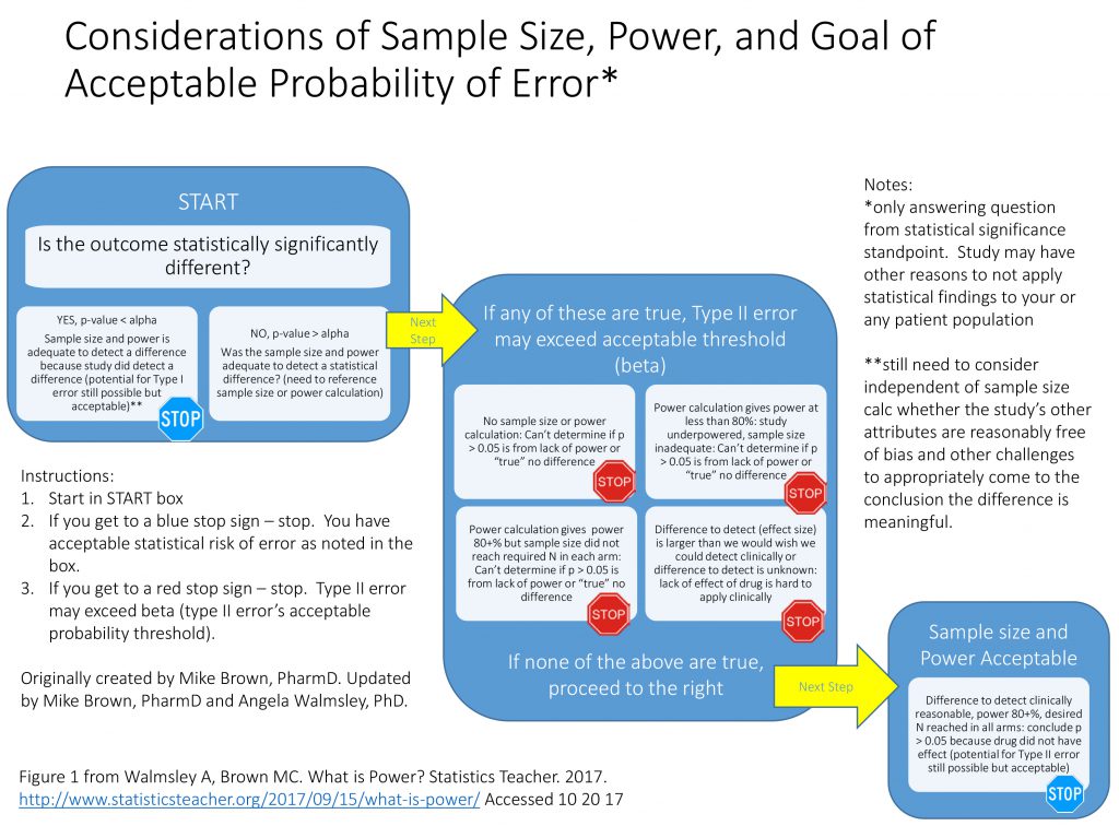
Having stated a little bit about the concept of power, the authors have found it is most important for students to understand the importance of power as related to sample size when analyzing a study or research article versus actually calculating power. We have found students generally understand the concepts of sampling, study design, and basic statistical tests, but sometimes struggle with the importance of power and necessary sample size. Therefore, the chart in Figure 1 is a tool that can be useful when introducing the concept of power to an audience learning statistics or needing to further its understanding of research methodology.

Figure 1 A tool that can be useful when introducing the concept of power to an audience learning statistics or needing to further its understanding of research methodology

This concept is important for teachers to develop in their own understanding of statistics, as well. This tool can help a student critically analyze whether the research study or article they are reading and interpreting has acceptable power and sample size to minimize error. Rather than concentrate on only the p-value result, which has so often traditionally been the focus, this chart (and the examples below) help students understand how to look at power, sample size, and effect size in conjunction with p-value when analyzing results of a study. We encourage the use of this chart in helping your students understand and interpret results as they study various research studies or methodologies.

Examples for Application of the Chart

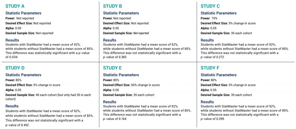
Imagine six fictitious example studies that each examine whether a new app called StatMaster can help students learn statistical concepts better than traditional methods. Each of the six studies were run with high-school students, comparing the morning AP Statistics class (35 students) that incorporated the StatMaster app to the afternoon AP Statistics class (35 students) that did not use the StatMaster app. The outcome of each of these studies was the comparison of mean test scores between the morning and afternoon classes at the end of the semester.

Statistical information and the fictitious results are shown for each study (A–F) in Figure 2, with the key information shown in bold italics. Although these six examples are of the same study design, do not compare the made-up results across studies. They are six independent pretend examples to illustrate the chart’s application.

Figure 2 Six fictitious example studies that each examine whether a new app called StatMaster can help students learn statistical concepts better than traditional methods (click to view larger)

In Study A, the key element is the p-value of 0.034. Since this is less than alpha of 0.05, the results are statistically significant and we can stop at the blue stop sign in the START box. While the study is still at risk of making a Type I error, this result does not leave open the possibility of a Type II error. Said another way, the power is adequate to detect a difference because they did detect a difference that was statistically significant. It does not matter that there is no power or sample size calculation when the p-value is less than alpha.

In Study B, the summaries are the same except for the p-value of 0.383. Since this is greater than the alpha of 0.05, we move in the chart to the large middle box to check for the presence or absence of acceptable Type II error. In this case, the criteria of the upper left box are met (that there is no sample size or power calculation) and therefore the lack of a statistically significant difference may be due to inadequate power (or a true lack of difference, but we cannot exclude inadequate power). We hit the upper left red STOP. Since inadequate power—or excessive risk of Type II error—is a possibility, drawing a conclusion as to the effectiveness of StatMaster is not statistically possible.

In Study C, again the p-value is greater than alpha, taking us back to the second main box. Unlike Study B, the presence of a desired power and sample size calculation allows us to avoid the red STOP in the upper left quadrant, but the power of 70% leaves us hitting the criteria of the upper right red STOP. With a power of 70%, our threshold of potential Type II error is 30% (1-0.7), which is above the traditionally acceptable 20%. The ability to draw a statistical conclusion regarding StatMaster is hampered by the potential of unacceptably high risk of Type II error.

In Study D, the p-value continues to be greater than alpha, but—unlike Study B and Study C—Study D has an appropriate power set at 80%. That is a good thing. The challenge becomes the desired sample size to meet this 80% power. Study D says it needs 40 subjects in each class to be confident of 80% power, but the study only has 35 subjects, so we hit the red STOP in the lower left quadrant. Because the desired sample size was not met, the actual power is less than 80%, leaving us effectively in the same situation as Study C—at risk of excessive Type II error beyond 20%.

In Study E, the challenges are more complex. With a p-value greater than alpha, we once again move to the middle large box to examine the potential of excessive or indeterminate Type II error. In this case, power (80%), alpha (0.05), and sample size (35 in each cohort) are all adequate. The effect size, however, is set at 50%.

While a 50% change in score would be of interest, it has two problems. First, it is likely that previous course offerings provide some estimate of performance in the absence of StatMaster, and—presuming it is even remotely close to the mean of 85% seen in Study E—a 50% increase would not be mathematically possible, making this an impractical effect size. Second, a sample size will provide adequate power to detect an effect size that is at least as big as the desired effect size or bigger, but not smaller. Reviewing the equation earlier in this manuscript provides the mathematical evidence of this concept.

So, while an effect size of 50% would be impressive—in the absence of a statistically significant outcome—Study E would not be certain to have adequate power to detect a smaller effect size, even though a smaller effect size might be of interest. Therefore, we are left at the red STOP sign in the lower right corner.

Note that, unlike the other red STOP signs, this example requires subjective judgment and is less objective than the other three paths to potentially exceeding acceptable Type II error. As noted earlier, this is a complex and challenging scenario to interpret, but is quite plausible (even common), and therefore included for consideration.

Our final example is Study F, in which we can progress to the box describing sample size and power as acceptable. The power (80%), desired effect size (5% change), and alpha (0.05) are all appropriate and the desired sample size (35 in each cohort) was met, leading us to the statistical conclusion that the absence of a statistically significant finding demonstrates no difference exists. Recognize that the potential for Type II error still exists, but it is no greater than 1 – power—or in this case 20% (1 – 0.8)—which is why it is deemed acceptable.

In conclusion, we encourage teachers to introduce the concept of power and its importance in evaluating statistical research. We are hopeful that both the sample scenarios and the flowchart are useful for both teachers and students as they explore the concept of power and how it relates to effect size, sample size, and significance level in general.